I’ve previously written on why I don’t want to rely on third party GUIs for managing my AWS services. Assuming I’ll be interacting with AWS through the SDK later on, I much prefer doing the initial setup using the SDK as well, to ensure I fully understand what I’ve done. Inpreviousposts, I’ve shown full console application examples on how to use the SDK for various tasks; however, creating a console application project, compiling and running it can be kind of cumbersome, especially if you’re just doing some quick testing or API exploration.
Enter LINQPad
If you haven’t tried LINQPad out before, go do it now! It’s an awesome scratchpad style application for writing and running C#/VB.NET/F# code, either as a single expression, a set of statements or a full application. There are also various plugins for easily connecting to databases, Azure services and lots more. Probably just a matter of time before someone writes a custom provider for AWS as well.
Getting started with the AWS SDK in LINQPad
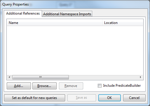
First up, you need to download and install the AWS SDK. Once installed, open LINQPad and press F4. In the following dialog, click Add…
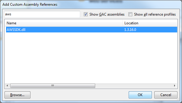
You can either browse to the AWSSDK.dll file manually, or you can pick it from the GAC – which would be the easiest option if you’re just doing some quick testing.
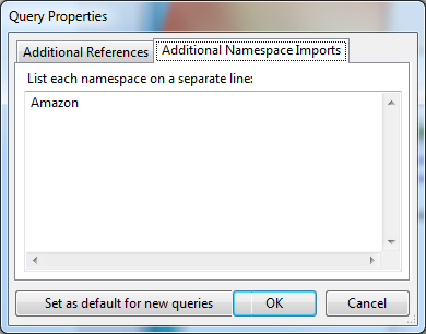
After adding it, as a final step, go to the Additional Namespace Imports tab and add Amazon to the list.
Discoverability
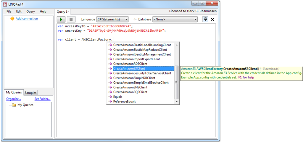
There are generally two ways to approach a new and unknown API. You could read the documentation, or you could just throw yourself at it, relying on intellisense. Unfortunately the free version of LINQPad does not come with intellisense/auto completion, however, at a price of $39 it’s a bargain.
Exception output
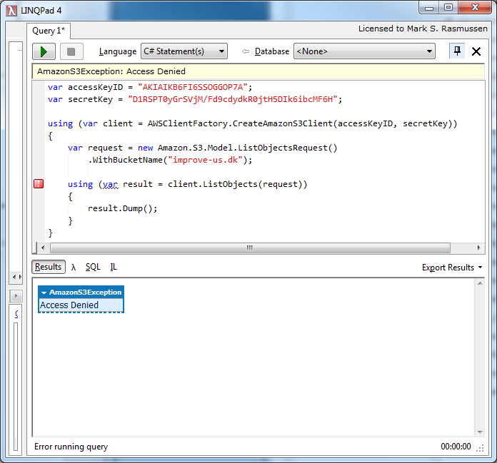
Inevitably, you’ll probably run into an exception or two. Take the following piece of code for example; it works perfectly, but I forgot to assign the IAM user access to the bucket I’m trying to interact with (and before you remind me to remove the keys, don’t worry, the IAM user was temporary and no longer exists):
var accessKeyID = "AKIAIKB6FI6SSOGGOP7A";
var secretKey = "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";

using (var client = AWSClientFactory.CreateAmazonS3Client(accessKeyID, secretKey))
{
	var request = new Amazon.S3.Model.ListObjectsRequest()
		.WithBucketName("improve-us.dk");

	using (var result = client.ListObjects(request))
	{
		result.Dump();
	}
}
What you’ll see is a clear notification saying an exception has occurred, as well as a repeated exception in the output pane:
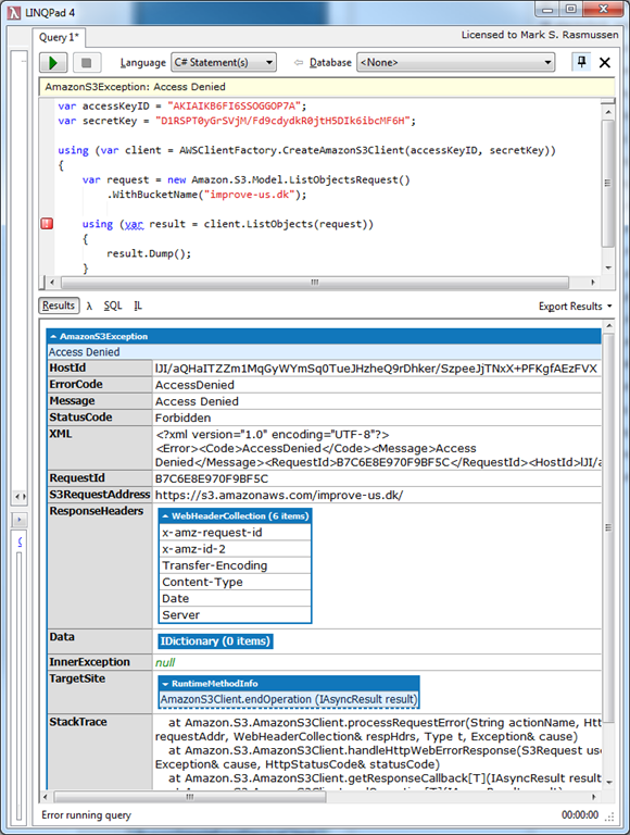
But look what happens once we expand the exception:
We get all of the output! Any object, returned or thrown from the code, will automatically be displayed in the output, and can easily be drilled into.
Dumping objects
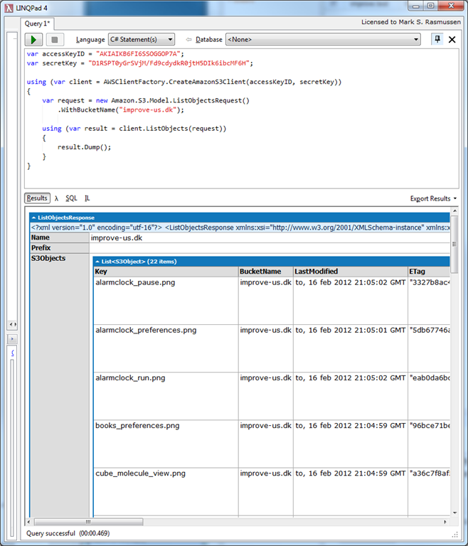
In case you’re code neither throws exceptions (by some miracle, in my case) nor returns objects, you can always call the .Dump() extension method on any object. Once I granted the IAM user the correct permissions, result.Dump() was called and the result of the ListObjectsRequest was output:
Once again it’s easy to drill down and see all of the properties of the result.
Conclusion
Adhering to my original statement of not liking third party GUIs, using tools like LINQPad is an excellent option for easily writing test code, without the added overhead of starting Visual Studio, compiling, running, etc. The output is neatly presented and really helps you to get a feeling for the API.
Just to finish off – LINQPad has plenty of uses besides AWS, this is just one scenario for which I’ve been using it extensively lately. I’m really considering creating a LINQPad provider for OrcaMDF as one of my next projects.
So what’s a multiplexer you ask? A multiplexer is an integrated circuit that takes a number of inputs and outputs a smaller number of outputs. In this case we’re aiming at creating a 4-to-1 multiplexer. As the name implies, it takes four inputs and outputs exactly one output, determined by a select input. Depending on the number of input lines, one or more select lines may be required. For 2n input lines, n select lines are needed. In hardware terms, this is basically the simplest of switches.
Creating a 2-to-1 multiplexer
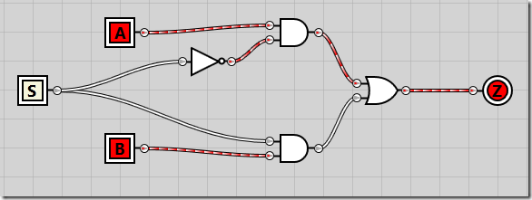
To start out easy, we’ll create a multiplexer taking two inputs and a single selector line. With inputs A and B and select line S, if S is 0, the A input will be the output Z. If S is 1, the B will be the output Z.
The boolean formula for the 2-to-1 multiplexer looks like this:
Z = (A ∧ ¬S) ∨ (B ∧ S)
If you’re not used to boolean algebra, it may be easier to see it represented in SQL:
SELECT @Z = (A & ~S) | (B & S)
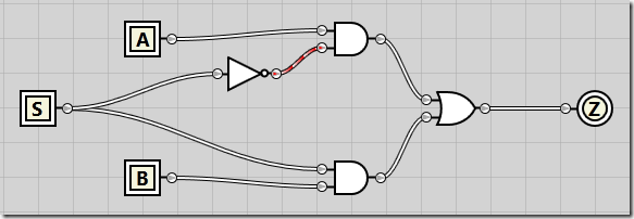
By ANDing A and B with NOT S and S respectively, we’re guaranteed that either A or B will be output. Creating the circuit, it looks like this:
If we enable both A and B inputs but keep S disabled, we see that the A input is passed all the way through to the Z output:
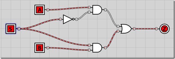
And if we enable the S selector line, B is passed through to Z as the output:
Creating a 4-to-1 multiplexer
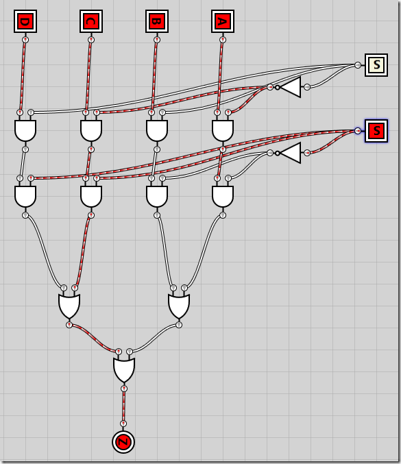
Now that we’ve created the simplest of multiplexers, let’s get on with the 4-to-1 multiplexer. Given that we have 22 inputs, we need two selector lines. The logic is just as before – combining the two selector lines, we have four different combinations. Each combination will ensure that one of the input lines A-D are passed through as the output Z. The formula looks like this:
The circuit is pretty much the same as in the 2-to-1 multiplexer, except we add all four inputs and implement the 4-input boolean formula, with S0 on top and S1 on bottom:
I’ll spare you a demo of all the states and just show all four inputs activated while the signal value of 0b10 results in C being pass through to Z as the result:
Combining two 4-to-1 multiplexers into an 8-to-1 multiplexer
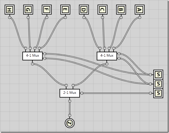
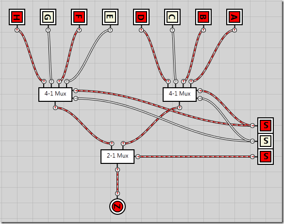
I’ll spare you the algebraic logic this time as it follows the same pattern as previously, except it’s starting to become quite verbose. In the following circuit I’ve taken the the exact 4-to-1 multiplexer circuit that we created just before, and turned it into an integrated circuit (just as I converted the 2-to-1 multiplexer into an integrated circuit). I’ve then added 8 inputs, A through H as well as three selector inputs, S0 through S2.
S0 and S1 are passed directly into each of the 4-1 multiplexers, no matter the value of S2. This means both 4-1 multiplexers are completely unaware of S2s existence. However, as the output from each of the 4-1 multiplexers are passed into a 2-1 multiplexer connected to the S2 selector line, S2 determines which of the 4-1 multiplexers get to deliver the output.
Here’s an example where S2 defines the output should come from the second (leftmost) 4-1 multiplexer, while the S0 and S1 selector lines defines the input should come from the second input in that multiplexer, meaning input F gets passed through as the result Z.
Combining two 8-to-1 multiplexers into a 16-to-1 multiplexer
Ok, let’s just stop here.Using the smaller multiplexers we can continue combining them until we reach the desired size.
After two months of on and off work, I finally merged the OrcaMDF compression branch into master. This means OrcaMDF now officially supports data row compression!
Supported data types
Implementing row compression required me to modify nearly all existing data types as compression changes the way they’re stored. Integers are compressed, decimals are variable length and variable length values are generally truncated instead of padded with 0’s. All previous data types implemented in OrcaMDF supports row compression, just as I’ve added a few. The current list of supported data types is as follows:
bigint
binary
bit
char
date
datetime
mal/numeric (including vardecimal, both with and without row compression)
image
int
money
nchar
ntext
nvarchar
smallint
smallmoney
text
time
uniqueidentifier
varbinary
varchar
Unicode compression
Nchar and nvarchar proved to be slightly more tricky than the rest as they use the SCSU unicode compression format. I found a single .NET implementation of SCSU, but while I was allowed to use the code, it didn’t come with a license and that’s a no go when I want to embed it in OrcaMDF. Furthermore had a lot of Java artifacts lying around (relying on goto for instance) that I didn’t fancy. I chose to implement my own SCSU decompression based on the reference implementation provided by Unicode, Inc. I’ve only implemented decompression to end up with a very slim and simple SCSU decompressor.
I’ll be posting a blog on the decompressor itself as it has some value as a standalone class outside of OrcaMDF.
Architecture changes
I started out thinking I’d be able to finish off compression support within a week or two, after all, it was rather well documented. It didn’t take long before it dawned upon me, just how many changes implementing compression would require. The record parser would obviously need to know whether the page was compressed or not. But where would it know that from? Previously all it got was a page pointer, now I had to lookup the compression (which varies by partition) metadata and make sure it was passed along all the way from the DataScanner to the page parser, to the record parser and onwards to the data type parsers.
I’ve had to implement multiple abstractions on top of the regular parsers to abstract away whether the records were stored in a compressed or non compressed format. Overall it’s resulted in a better architecture, but it took a lot more work than expected. Actually parsing the compressed record format was the smallest part of the ordeal – the documentation was spot on and it’s a simple format. The data types however, that took some more work until I had the format figured out.
Taking it for a spin
As always, the code is available at Github, feel free to take a look! If you’re not the coding type, I’ve also uploaded the binary download (dated 2012-02-06) of the OrcaMDF Studio, a GUI built on top of OrcaMDF.
Stats
Being a lover of numbers myself, I love looking at statistics. Here’s a couple of random stats from OrcaMDF:
123 commits, the first one being made on April 15th 2011 – that’s almost a year ago!
~11.700 lines of C# code (excluding blanks).
~1000 lines of comments.
~35% of the code is dedicated to testing, with a test suite comprising of over 200 tests.
Ohloh estimates OrcaMDF has a development cost of $144,090 – makes me wonder if not my time would be better spent elsewhere…
Most people can do simple decimal addition in their heads, and even advanced addition using common rules like carrying. Here’s how we’d add 6 + 7:
1 6+ 7
---- 13
Adding 6+7 gives a result of 3, with a 1 as a carry. In the final step, the 1 carry simply falls down as a 10 on the result, giving 10 + 3 = 13 as the final result.
It may seem extensive to go through this for such a simple operation, but it’s quite important to know of the carry method when we go on.
Binary addition
Just as we added two decimal numbers, we can do the exact same in binary. In binary 6 is represented as 0b110 while 7 is represented as 0b111. Take a look:
First we add the first (rightmost) column, resulting in a 0b1 in the sum:
110+ 111
------ 1
Next up we add the second column. In this case the two ones produce the result 0b10 – meaning we’ll get a sum of 0b0 and a carry of 0b1:
110+ 111
------ 01
Then we add the third column. Ignoring the carry, 0b1 + 0b1 gives a sum of 0b10. Adding the 0b1 we had in carry, we get 0b11 – resulting in a sum of 0b1 as well as a carry of 0b1:
11 110+ 111
------ 101
And finally we add the final column, in this case containing nothing but the carry:
11 110+ 111
------ 1101
And there we go – 0b1101 = 13 = 6 + 7.
Implementing a simple ALU that does addition
Now that we can do binary addition by hand, lets recreate a very simple arithmetic logic unit that’ll do the same. The ALU is at the very core of the CPU that’s powering your machine right now. It’s the hearth that does all of the arithmetic and logical operations that are required to run the computer.
In the following I will generally talk of single bits as being enabled/positive/true/1 or being disabled/negative/false/0. All four designations mean the same and will be used depending on the context.
The half adder
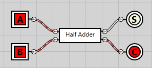
The first step is to implement what’s known as a half adder#Half_adder). This is the circuit that takes two bits and adds them together. The result is a sum value as well as a carry. Both can be either 0 or 1.
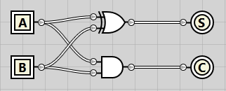
In the following circuit we get two inputs from the left, bits A and B. Both A and B are connected to an XOR gate. The XOR gate (top) gives an output of 1 iff (if and only if) only one of the inputs have a value of 1. If A and B have the same value, it gives a result of 0. This is just what we need for the sum – remember, 0b1 + 0b1 gave a result of 0b10 – a sum of 1 and a carry of 0. The XOR gate is thus used to calculate the sum – denoted S in the circuit below.
Both A and B are connected to an AND gate as well (bottom). The AND gate gives a result of 1 iff both A and B are 1, in all other cases it gives a result of 0. This is just what we need – if both A and B are 1, it means we get an output of 1 – the carry.
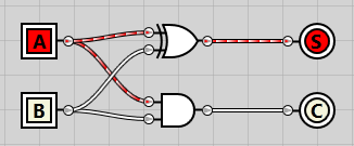
If we enable A, we see how the signal propagates through the XOR gate and results in an enabled sum:
The result is exactly the same if we just enable B instead:
And finally, if we enable both, we get a disabled sum but an enabled carry instead:
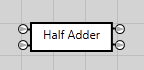
As we’ll be reusing the half adder in the next circuit, I’ve converted it into an integrated circuit (IC). On the left we have the input bits A and B on top & bottom respectively. On the right we have the sum on top and the carry at the bottom.
Having created the half adder IC, we can now simplify our circuit somewhat:
The full adder
At this point we have a fully working ALU capable of adding two 1-bit numbers and outputting a 2-bit result. As most computers today are either 32-bit or 64-bit, we obviously need to expand our ALU’s capabilities. Let’s work towards making it accept two 2-bit inputs instead.
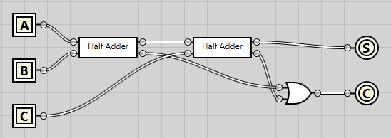
To do so we first need to create another component, the full adder#Full_adder). While the half adder is great for working with just two inputs, to calculate the next column we need to take three inputs – bits A and B, as well as the potential carry C. The result, as before, should still be a sum as well as a carry.
Technically what we’re creating is called a 1-bit full adder, since it’s able to add two 1-bit numbers while also respecting the carry input.
In the following circuit we use two of the half adder IC’s that we created before. Bits A and B are hooked into the first one, while the carry bit is hooked into the second half adder. The sum from the first half adder is used as the second input to the second half adder.
The end sum is a direct sum from both the half adders. For the sum to be enabled, both half adders must produce an enabled sum. Both carry outputs are connected to an OR gate. As the name implies, the OR gate will output a positive result if either of the inputs are enabled.
If we enabled the A bit, the sum passes right through both half adders and results in a positive sum output:
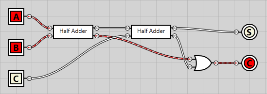
If we enabled both A and B, the first half adder gives a carry output, which passes right through the OR gate and results in a positive carry output:
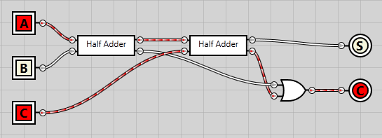
And finally, if we enable the input carry bit as well, we get a carry output from the first half adder and a sum output from the second one:
The way the circuit is constructed, it doesn’t matter which of the bits are enabled, only the amount of them. If one is enabled, we get a positive sum. Two enabled results in a positive carry. And finally, if all three are enabled, we get a positive sum as well as a positive carry.
Just to demonstrate, we can disable the B input and get the same positive carry result as we got with the A and B bits enabled:
Just as we can disabled all but the carry input and get a sum output, just like when only the A bit was enabled:
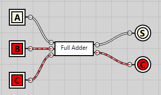
Having created this circuit, we can now convert it into a full adder IC and simplify our diagram:
Chaining 1-bit full adders to create a 3-bit ripple carry adder
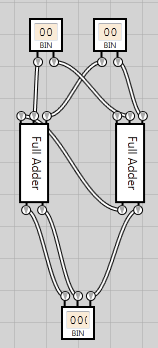
Now that we’re able to easily add two 1-bit numbers using our full adder, let’s try and chain them up so we can add two 2-bit numbers.
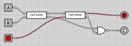
In the following diagram we have two 2-bit inputs. The first output bit of both inputs are connected to the A and B inputs on the first full adder (rightmost one). Likewise, the second output bits from each input is connected to the A and B inputs on the second full adder. The carry output from the first full adder is connected to the carry input on the second full adder.
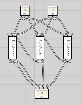
Now, we started out wanting to add the numbers 6 and 7. To do so, we need a 3-bit adder so we can express the input numbers 6 and 7, both requiring three input bits.
At this point it’s a trivial operation to extend the adder with one more bit. We simply connect each output bit from the first input to the A bits on each full adder. Likewise we connect each output bit on the second input to the B input bits on each full adder. The carry from the first full adder is added as carry input to the second, and likewise for the second and third full adders.
By using the decimal inputs we can now type the input numbers 6 and 7 and see our whole circuit in action, providing the correct output of 13:
And there we go, we’ve now created a 3-bit ripple carry adder#Ripple_carry_adder).
Conclusion
I’m sure (read: hope) I’m not the only one having the nightmare of an apocalyptic event occurring here on Earth. Imagine the scenario, you’ve got all of the materials in the world as well as all the manpower you need. Unfortunately, you’re the only computer scientist that’s survived. Given time, manpower and materials, would you be able to rebuild the computer as we know it today?
Each layer you peel off of the computer arms you with more knowledge and capability, not just at that layer, but at all of the layers that lie above. Knowing about gate logic enables you to understand so much more of how the CPU works as well as what’s actually being performed once you write “int x = 6+7;” in your application (assuming you also know about all of the layers between the logic gates and your C#/other high level code).
Naturally there are more layers to peel. For instance, you could create your own XOR/AND/OR gates using the base NAND gate. And you could create your own NAND gates using nothing but interconnected transistors. And you could create your own transistors using… You get the point.
I can’t help but feel in total awe of the amount of technology that’s packed in each and every CPU that’s shipped to a home computer somewhere. Experimenting with electrical circuits is lots of fun, and you learn loads from it.
If you want to try it out for yourself, go grab a copy of Steve Kollmansbergers (free) open source Logic Gate Simulator.
Several times a day I’d get an error report email noting that the following exception had occurred in our ASP.NET 4.0 application:
System.Web.HttpException (0x80004005) at System.Web.CachedPathData.ValidatePath(String physicalPath) at System.Web.HttpApplication.PipelineStepManager.ValidateHelper(HttpContext context)
The 80004005 code is a red herring – it’s used for lots of different errors and doesn’t really indicate what’s wrong. Besides that, there’s no message on the exception, so I was at a loss for what might’ve caused it.
We have several 100k’s of visitors each day and I only got 5-10 of these exceptions a day, so it wasn’t critical. Even so, I don’t like exceptions being thrown without reason. After much digging (and cursing at the combination of our error logging and gmail trimming the affected URL’s), I discovered the cause.
All of the URL’s had an extra %20 at the end – caused by others linking incorrectly to our site.
After a short bit of Googling, I found the new RelaxedUrlToFileSystemMapping httpRuntime attribute in .NET 4.0. And sure enough, setting it to false (or letting it have it’s default false value), an exception is thrown when I add %20 to the URL. Once set to true, everything works as expected.
Though I got the problem solved, I would’ve appreciated a more descriptive exception being thrown.
While working on row compression support for OrcaMDF, I ran into some challenges when trying to parse integers. Contrary to normal non-compressed integer storage, these are all variable width – meaning an integer with a value of 50 will only take up one byte, instead of the usual four. That wasn’t new though, seeing as vardecimals are also stored as variable width. What is different however is the way the numbers are stored on disk. Note that while I was only implementing row compression, the integer compression used in page compression is exactly the same, so this goes for both types of compression.
Tinyint
Tinyint is pretty much identical to the usual tinyint storage. The only exception being that a value of 0 will take up no bytes when row compressed, where as in non-compressed storage it’ll store the value 0x0, taking up a single byte. All of the integer types are the same regarding 0-values – the value is indicated by the compression row metadata and thus requires no actual value stored.
Smallint
Let’s start out by looking at a normal non-compressed smallint, for the values –2, –1, 1 and 2. As mentioned before, 0 isn’t interesting as nothing is stored. Note that all of these values are represented exactly as they’re stored on disk – in this case they’re stored in little endian.
-2 = 0xFEFF
-1 = 0xFFFF1 = 0x01002 = 0x0200
Starting with the values 1 and 2, they’re very straightforward. Simply convert it into decimal and you’ve got the actual number. –1 however, is somewhat different. The value 0xFFFF converted to decimal is 65.535 – the maximum value we can store in an unsigned two-byte integer. The SQL Server range for a smallint is –32.768 to 32.767.
Calculating the actual values relies on what’s called integer overflows. Take a look at the following C# snippet:
If we start with the value 0 and add the maximum value for a signed short, 32.767, we obviously end up with just that – 32.767. However, if we add 32.768, which is outside the range of the short, we rollover and end up with the smallest possible short value. Since these are constant numbers, the compiler won’t allow the overflow – unless we encapsulate our code in an unchecked {} section.
You may have heard of the fabled sign bit. Basically it’s the highest order bit that’s being used to designate whether a number is positive or negative. As special sounding as it is, it should be obvious from the above that the sign bit isn’t special in any way – though it can be queried to determine the sign of a given number. Take a look at what happens to the sign bit when we overflow:
For the number to become large enough for it to cause an overflow, the high order “sign bit” needs to be set. It isn’t magical in any way, it’s simply used to cause the overflow.
OK, so that’s some background information on how normal non-compressed integers are stored. Now let’s have a look at how those same smallint values are stored in a row compressed table:
-2 = 0x7E
-1 = 0x7F1 = 0x812 = 0x82
Let’s try and convert those directly to decimal, as we did before:
Obviously, these are not stored the same way. The immediate difference is that we’re now only using a single byte – due to the variable-width storage nature. When parsing these values, we should simply look at the number of byte stored. If it’s using a single byte, we know it’s in the 0 to 255 range (for tinyints) or –128 to 127 range for smallints. Smallints in that range will be stored using a single signed byte.
If we use the same methodology as before, we obviously get the wrong results.1 <> 0 + 129. The trick in this case is to treat the stored values as unsigned integers, and then minimum value as the offset. That is, instead of using 0 as the offset, we’ll use the signed 1-byte minimum value of –128 as the offset:
Aha, so that must mean we’ll need to store two bytes as soon as we exceed the signed 1-byte range, right? Right!
One extremely important difference is that the non-compressed values will always be stored in little endian on disk, whereas the row compressed integers are stored using big endian! So not only do they use different offset values, they also use different endianness. The end result is the same, but the calculations involved are dramatically different.
Int & bigint
Once I figured out the endianness and number scheme of the row-compressed integer values, int and bigint were straightforward to implement. As with the other types, they’re still variable width so you may have a 5-byte bigint as well as a 1-byte int. Here’s the main parsing code for my SqlBigInt type implementation:
The value variable is a byte array containing the bytes as stored on disk. If the length is 0, nothing is stored and hence we know it has a value of 0. For each of the remaining valid lengths, it’s simply a matter of using the smallest representable number as the offset and then adding the stored value onto it.
For non-compressed values we can use the BitConverter class directly as it expects the input value to be in system endianness – and for most Intel and AMD systems, that’ll be little endian (which means OrcaMDF won’t run on a big endian system!). However, as the compressed values are stored in big endian, I have to remap the input array into little endian format, as well as pad the 0-bytes so it matches up with the short, int and long sizes.
For the shorts and ints I’m reading unsigned values in, as that’s really what I’m interested in. This works since int + uint is coerced into a long value. I can’t do the same for the long’s since there’s no data type larger than a long. For the maximum long value of 9.223.372.036.854.775.807, what’s actually stored on disk is 0xFFFFFFFFFFFFFFFF. Parsing that as a signed long value using BitConverter results in the value –1 due to the overflow. Wrong as that may be, it all works out in the end due to an extra negative overflow:
As usual, I’ve had a lot of fun trying to figure out how the bytes on disk ended up as the values I saw when performing a SELECT query. It doesn’t take long to realize that while the excellent Internals book really takes you far, there’s so much more to dive into.
To my big surprise, I’ve got another chance at speaking at SQLBits – I must’ve done something right after all :)
I will once again be presenting a session based on my work with OrcaMDF. Here’s the abstract:
Think SQL Server is magical? You’re right! However, there’s some sense to the magic, and that’s what I’ll show you in this level 500 deep dive session. Through my work in creating OrcaMDF, an open source parser for SQL Server databases, I’ve learned a lot of internal details for the SQL Server database file format. In this session, I will walk you through the internal storage format of MDF files, how we might go about parsing a complete database ourselves, using nothing but a hex editor. I will cover how SQL Server stores its own internal metadata about objects, how it knows where to find your data on disk, and once it finds it, how to read it. Using the knowledge from this session, you’ll find it much easier to predict performance characteristics of queries since you’ll know what needs to be done.
The basis of the session is the same as the one I gave last year. However, based on the feedback I got, as well as the work I’ve done with OrcaMDF since then, I’ll be readjusting the content a bit. I’ll not be covering disaster recovery, just as I’ll trim some sections to leave room for some new stuff like compression internals.
Just as last time, the session is meant to inspire, not to teach. There’ll be far too much content to understand everything during the session. My hope is to reveal how SQL Server is really governed by a relatively small set of rules – and once you know those, you’ve got a powerful tool to add to your existing arsenal.
Every night at around 2AM I get an email from my best friend, confirming that she’s OK. It usually looks something like this:
JOB RUN: ‘Backup.Daily’ was run on 04-08-2011 at 02:00:00 DURATION: 0 hours, 5 minutes, 57 seconds STATUS: Succeeded MESSAGES: The job succeeded. The Job was invoked by Schedule 9 (Backup.Daily (Mon-Sat)). The last step to run was step 1 (Daily).
Just the other night, I got one that didn’t look right:
DURATION: 4 hours, 3 minutes, 32 seconds
Looking at the event log revealed a symptom of the problem:
SQL Server has encountered 2 occurrence(s) of I/O requests taking longer than 15 seconds to complete on file [J:XXX.mdf] in database [XXX] (150). The OS file handle is 0x0000000000003294. The offset of the latest long I/O is: 0x00000033da0000
Our databases were the same, the workload was the same. The only teeny, tiny little thing that had changed was that I’d moved all of the data files + backup drive onto a new SAN. Obviously, that’s gotta be the problem.
Broadcom, how I loathe thee!
Through some help on #sqlhelp and Database Administrators, I managed to find the root cause as well as to fix it. For a full walkthrough of the process, please see my post on Database Administrators.
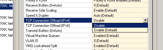
Mark Storey-Smith ended up giving the vital clue – a link to a post by Kyle Brandt which I clearly remember reading earlier on, but didn’t suspect was applicable to my situation. I ended up disabling jumbo frames, large send offload (LSO) and TCP connection offload (TOE), and lo and behold, everything was running smoothly. By enabling each of the features individually I pinpointed the issue to the Broadcom TOE feature on the NICs. Once I enabled TOE, my IO requests were stalling. As soon as I disabled TOE, everything ran smoothly.
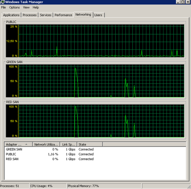
After disabling TOE on both NICs, my backups went from looking like this:
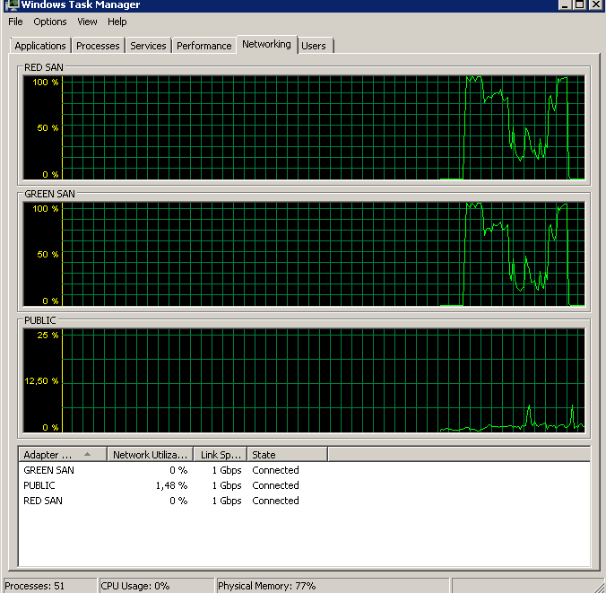
To this:
At this point the backup timing was back on track and the event log was all green. I did use the same Broadcom NICs with TOE enabled for the previous SAN, so obviously something must have triggered the issue, whether it’s a problem between the new switches, the drivers, cables, I have no idea. All I know is that I’m apparently not the first to suffer similar issues with Broadcom NICs and I know for sure that I’ll get Intels in my next servers.
Having presented at Miracle Open World back to back in 2010 and 2011, I’m excited to announce I’ll also be present in 2012! Not only will I be presenting, I’ll be presenting a full day track.
I’ve been continually improving my original internals training day that I presented at SQLBits. At MOW, I’ll be presenting the evolved session, which now also includes compression internals. As the allotted time at MOW is slightly shorter than at SQLBits, and I have slightly more material, expect to bring coffee :)
In this post I’ll do a deep dive into how vardecimals are stored on disk. For a general introduction to what they are and how/when to use them, see this post.
Is vardecimal storage enabled?
First up, we need to determine whether vardecimals are enabled, since it completely changes the way decimals are stored on disk. Vardecimal is not a type itself, so all columns, whether stored as decimals are vardecimals share the same system type (106). Note that in SQL Server, numeric is exactly the same as decimal. Anywhere I mention decimal, you can substitute that with numeric and get the same result.
Provided SQL Server is running, you can execute the following to determine the vardecimal status of any given table:
Normal decimal columns are stored in the fixed length portion of a record. This means all that’s actually stored is the data itself. There is no need for length information as the number of required storage bytes can be calculated exclusively by the use of metadata. Once you enable vardecimals, all decimals are no longer stored in the fixed length portion of the record, but as a variable length field instead.
Storing the decimal as a variable length field has a couple of implications:
We can no longer statically calculate the number of bytes required to store a given value.
There’s a two byte overhead for storing the record offset value in the variable length offset array.
If the record previously had no variable length records, that overhead is actually four bytes since we also need to store the number of variable length records in the record offset array.
The actual value of the decimal has a variable amount of bytes that we need to decipher.
What does the vardecimal value consist of?
Once we’ve parsed the record and thereby retrieved the vardecimal value bytes from the variable length portion of the record, we need to parse it. There will always be at least two bytes for the value, though there can be up to 20 at most.
Where normal decimals are basically stored as one humongous integer (with the scale metadata defining the decimal position), vardecimals are stored using scientific notation. Using scientific notation, we need to store three different values:
The sign (positive/negative).
The exponent.
The mantissa.
Using these three components, we can calculate the actual number using the following formula:
(sign) * mantissa * 10<sup>exponent</sup>
Example
Assume we have a vardecimal(5,2) column and we store the value 123.45. In scientific notation, that would be expressed as 1.2345 * 102. In this case we have positive sign (1), an mantissa of 1.2345 and an exponent of 2. SQL Server knows that the mantissa always has a fixed decimal point after the first digit, and as such it simply stores the integer value 12345 as the mantissa. While the exponent is 2, SQL Server knows we have a scale of 2 defined, and it subtracts that from the exponent and thus stores 0 as the actual exponent.
Once we read it, we end up with a formula like this for calculating the mantissa (note that at this point we don’t care if the mantissa is positive or negative – we’ll take that into account later):
mantissa / 10<sup>floor(log10(mantissa))</sup>
And plotting in our values, we get:
12345 / 10<sup>floor(log10(12345))</sup>
Through basic simplification we get:
12345 / 10<sup>4</sup>
Which finally ends up in the scientific notation version of the mantissa:
1.2345
So far so good – we now have the mantissa value. At this point we need just two things – to apply the sign and to move the decimal into the right position by factoring in the exponent. As SQL Server knows the scale is 2, it stores an exponent value of 2 instead of 4, in effect subtracting the scale from the exponent value – enabling us to ignore the scale and just calculate the number directly.
And thus we have all we need to calculate the final number:
The very first byte of the value contains the sign and the exponent. In the previous sample, the value takes up four bytes (plus an additional two for the offset array entry):
0xC21EDC20
If we take a look at just the first byte, and convert it to binary, we get the following:
Hex: C2
Bin: 11000010
The most significant bit (the leftmost one), or bit 7 (0-indexed) is the sign bit. If it’s set, the value is positive. If it’s not set, it’s negative. Since it has a value of 1, we know that the result is positive.
Bits 0-6 is a 7-bit value containing the exponent. A normal unsigned 7-bit value can contain values from 0 to 127. As the decimal data type has a range of –1038+1 to 1038-1, we need to be able to store negative numbers. We could use one of those 7 bits as a sign bit, and then store the value in just 6 bits, allowing a range from –64 to 63. SQL Server however does use all 7 bits for the value itself, but stores the value offset by 64. Thus, an exponent value of 0 will store the value 64. An exponent of –1 will store 63 while an exponent of 1 will store 65, and so forth.
In our sample, reading bits 0-6 gives the following value:
0b11000010 = 66
Subtracting the offset of 64 leaves us with an exponent value of 2.
Mantissa chunk storage
The remaining bytes contain the mantissa value. Before we get started, let’s convert them into binary:
Hex: 1E       DC       20

Bin: 00011110 11011100 00100000
The mantissa is stored in chunks of 10 bits, each chunk representing three digits in the mantissa (and remember, the mantissa is just one large integer – it’s not until later that we begin to think of it as a decimal pointer number). Splitting the bytes into chunks gives us the following grouping:
Hex:   1E       DC       20
Bin:   00011110 11011100 00100000

Chunk: 1          2
In this case, SQL Server wastes 4 bits by using a chunk size that doesn’t align with the 8-bit byte size. This begs the question, why choose a chunk size of just exactly 10 bits? Those 10 bits are required to represent all possible values of a three-digit integer (0-999). What if we instead wanted to use a chunk size representing just a single digit?
In that case, we’d need to represent the values 0-9. That requires a total of 4 bits (0b1001 = 9). However, using those 4 bits, we can actually represent a range spanning from 0 to 15 – which means we’re wasting 6 of those values as they’ll never be needed. In percentages, we’re wasting 6/16 = 37.5%!
Let’s try and plot some different chunk sizes into a graph:
We see that chunk sizes of both 4 and 7 have massive waste compared to a chunk size of 10. At 20 bits, we’re getting closer, but still waste twice as much as at 10.
Now, waste isn’t everything. For compression, ideally we don’t want to use more digits than absolutely necessary. With a chunk size of 10, representing 3 digits, we’re wasting two digits for values in the range of 0-9. However, for numbers in the range 100-999, we’re spot on. If we were to use a chunk size of 20 bits, representing 6 digits per chunk, we’d be wasting bytes for values 0-99999, while we’d be spot on for values 1000000-999999. Basically it’s a tradeoff – the higher the granularity, with the least amount of waste, the better. The further to the right we go in the graph, the less the granularity. With this, it seems obvious that a chunk size of 10 bits is an excellent choice – it has the lowest amount of waste with a suitable amount of granularity at 3 digits.
There’s just one more detail before we move on. Imagine we need to store the mantissa value 4.12, effectively resulting in the integer value 412.
Dec: 412
Bin: 01100111 00
Hex: 67       0
In this case, we’d waste 8 bits in the second byte, since we only need a single chunk, but we need two bytes to represent those 10 bits. In this case, given that the last two bits aren’t set, SQL Server will simply truncate that last byte. Thus, if you’re reading a chunk and you run out of bits on disk, you can assume that the remaining bits aren’t set.
Parsing a vardecimal value
Finally – we’re ready to actually parse a stored vardecimal (implemented in C#)! We’ll use the previous example, storing the 123.45 value in a decimal(5,2) column. On disk, we read the following into a byte array called value:
Hex: C2       1E       DC       20
Bin: 11000010 00011110 11011100 00100000
Reading the sign bit
Reading the sign bit is relatively simple. We’ll only be working on the first byte:
Hex: C2       1E       DC       20
Bin: 11000010 00011110 11011100 00100000
By shifting the bits 7 spots to the right, all we’re left with is the most significant bit, the least significant position. This means we’ll get a value of 1 is the sign is positive, and 0 if it’s negative.
decimal sign = (value[0] >> 7) == 1 ? 1 : -1;
Reading the exponent
The next (technically these bits come before the sign bit) 7 bits contain the exponent value.
Hex: C2 1E DC 20
Bin: 1100001000011110 11011100 00100000
Converting the value 0b1000010 into decimal yields the decimal result 66. As we know the exponent is always offset by a value of 64, we need to subtract 64 from the stored value to get to the actual exponent value:
Next up is the mantissa value. As mentioned, we need to read it in chunks of 10 bits, while taking care of there potentially being some truncated bits.
First, we need to know how many bits there are available. Doing this is straightforward – we simply multiply the number of mantissa bytes (which is all of the bytes, except one) by 8:
int totalBits = (value.Length - 1) * 8;
Once we know how many bits are available (3 bytes of 8 bits = 24 in this case), we can calculate the number of chunks:
int mantissaChunks = (int)Math.Ceiling(totalBits / 10d);
Since each chunk takes up 10 bits, we just need to divide the total number of bits by 10. If there’s padding at the end, to match a byte boundary, it’ll all be 0’s and won’t change the end result. Thus for a 2-byte mantissa we’ll have 8 bits to spare, which will all be non-significant 0’s. For a 3-byte mantissa we’ll have 4 bits to spare – once again adding 0 to the total mantissa value.
At this point we’re ready to read the chunk values. Before doing so, we’ll allocate two variables:
decimal mantissa = 0;
int bitPointer = 8;
The mantissa variable contains the cumulative mantissa value, accumulating value each time we read a new 10-bit chunk. The bitPointer is a pointer to the index of the bit currently being. As we’re not going to read the first byte, we’ll start this one off at bit index 8 (0-based, thus bit index 8 = the first bit of the second byte).
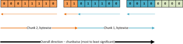
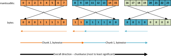
Looking at the bits as one long stream makes it look simple – we just read from left to right, right? Not quite. As you may remember, (visually) the rightmost bit is the least significant, and is thus the first one we should read. However – we need to read one byte at a time. As such, the overall direction is left-to-right, chunkwise. Once we get to any given chunk, we need to read one byte at a time. Bits 1-8 in the first chunk are read from the first byte, while bits 9-10 are read from the second byte, following the orange arrows in the figure (byte read order following the large ones, individual byte bit read order following the smaller ones):
To easily access all of the bits, and to avoid doing a lot of manual bit shifting, I initialize a BitArray that contains all of the data bits:
var mantissaBits = new BitArray(value);
Using this, you have to know how the bit array maps into the bytes. Visually, it looks like this, the mantissaBits array index being on top:
I know this may seem complex, but it’s all just a matter of knowing which pointers point to which values. Our source is the array of bytes. The way we access the individual bits is through the mantissaBits array, which is just one big array of pointers to the individual bits.
Looking at just the first 8 bits, the manitssaBits array aligns nicely with the direction we need to read. The first entry (mantissaBits[0]) points to the first/rightmost bit in the first byte. The second entry points to the second bit we need to read, and so forth. Thus, the first 8 bits are straightforward to read. The next two however, they require us to skip 6 entries in the mantissaBits array so we read index 14 and 15, as those point to the last two bits in the next byte.
Reading the second chunk, we have to go back and read bit index 8-13 and then skip to index 20-23, ignoring entries 16-19 as they’re just irrelevant padding. This is rather tricky to get right. Fortunately we can freely choose to read the bits from the least significant to the most significant, or the other way around.
Let’s first look at the implementation:
for (int chunk = mantissaChunks; chunk > 0; chunk--)
{
// The cumulative value for this 10-bit chunkdecimal chunkValue = 0;
// For each bit in the chunk, shift it into position, provided it's setfor (int chunkBit = 9; chunkBit >= 0; chunkBit--)
{
// Since we're looping bytes left-to-right, but read bits right-to-left, we need// to transform the bit pointer into a relative index within the current byte.int byteAwareBitPointer = bitPointer + 7 - bitPointer % 8 - (7 - (7 - bitPointer % 8));
// If the bit is set and it's available (SQL Server will truncate 0's), shift it into positionif (mantissaBits.Length > bitPointer && mantissaBits[byteAwareBitPointer])
chunkValue += (1 << chunkBit);
bitPointer++;
}
// Once all bits are in position, we need to raise the significance according to the chunk// position. First chunk is most significant, last is the least significant. Each chunk// defining three digits.
mantissa += chunkValue * (decimal)Math.Pow(10, (chunk - 1) * 3);
}
The outer for loop loops through the chunks, going from the most significant to the least significant chunk. In this case we’ll first iterate over chunk 2, then chunk 1.
The chunkValue variable holds the total value for the chunk that we’re currently reading. We’ll be shifting bits into the variable until we have parsed all 10 bits.
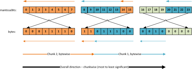
Next, we loop from the most significant bit to the least significant bit (that is, going from the chunkBit values 9 through 0). By reading the most significant bit first, basically reading the values backwards, we avoid having to skip inside the individual bytes. We’ll always read the bits going from right to left in the mantissaBits array, following the top arrows like this:
Though we do read each byte backward, everything else just follows a natural path, which makes parsing a lot easier.
The byteAwareBitPointer variable is the index in our mantissaBits array from where we’ll read the current value. The calculation ensures we read each byte starting from the top mantissaBits index to the lower one. The first chunk is read in the following mantissaBit index order:
7, 6, 5, 4, 3, 2, 1, 0, 15, 14
And the second chunk is read in the following mantissaBit order:
13, 12, 11, 10, 9, 8, 23, 22, 21, 20
Once we’ve read a specific bit, we shift it into position in the chunkValue variable – though only if it’s set and it’s available (that is, it hasn’t been zero-truncated).
Once all bits have been shifted into position, we apply the chunk significance to the value. In our case, storing the value 12345, we’re actually storing the value 123450 (since each chunk stores three digits, it’ll always be a multiple of 3 digits). The first read chunk (chunk 2) contains the value 123, which corresponds to the value 123000. The second read chunk (chunk 1) contains the value 450. Multiplying by 10(chunk–1)<3 ensures we get the right order of magnitude (x1000 for chunk 2 and x1 for chunk 1*). For each chunk iteration, we add the finalized chunk value to the total mantissa sum.
Once we have the integer based mantissa value of 123450, we need to insert the decimal point, using the following formula:
This results in the mantissa having a value of 1.2345
Mantissa parsing performance
Before you beat me to it – this implementation is far from fast. To start with, we could easily shift whole groups of bits into position instead of just one at a time. That’d ensure each chunk would take no more than two shifting operations, instead of ~10 in this implementation. However, my goal for this implementation is code clarity first and foremost. I’m nowhere near the point where I want to look at optimizing OrcaMDF for speed.
Putting it all together
Once we have the sign, the exponent and the mantissa, we simply calculate the final value like so:
Vardecimal was the only option for built-in compression back in SQL Server 2005 SP2. Since 2008, we’ve had row & page compression available (which both feature a superset of the vardecimal storage format). Ever since the release of row & page compression, Microsoft has made it clear that vardecimal is a deprecated feature, and it will be removed in a future version. Since vardecimal requires enterprise edition, just like row & page compression, there’s really no reason to use it, unless you’re running SQL Server 2005, or unless you have a very specific dataset that would only benefit from compressing the decimals and no other values.
Knowing how the vardecimal storage format works is a great precursor for looking at compression internals – which I’ll be writing about in a later post – and I’ll be presenting on it at the 2012 Spring SQL Server Connections.